Fractals: More L-Systems
Mon 13 January 2020 by A Silent Llama
This post follows on from the previous posts on fractals.
Fractals with JSON
It’s a little annoying to have to recompile our program for every change. It would be better to define our pattern and rule in a seperate file and pass them in. Let’s first create a FractalDefinition struct that we can use to define how we want to draw things.
Create a fractal_def.rs file and add the following:
// fractal_def.rs
use serde::Deserialize;
use std::collections::HashMap;

#[derive(Deserialize)]
pub struct FractalDefinition {
    pub axiom: String,
    pub rules: HashMap<char, String>,
    pub iterations: u32,
    pub angle: f32,
    pub forward: f32,
    pub start_x: u32,
    pub start_y: u32,
    pub start_angle: f32,
    pub width: Option<u32>,
    pub height: Option<u32>,
}
We’ll need to change our Cargo.toml as well:
[dependencies]
image = "*"
imageproc = "*"
serde = { version = "1.0", features = ["derive"] }
serde_json = "1.0"
We’ve added the serde Rust library. This library makes it easy to serialize and deserialize data. We’ll use it to load our fractal definitions from json files. Let’s add in some code to read the definition from the command line:
// main.rs
// -- snip --
use fractal_def::FractalDefinition;
use std::env;
use std::fs::File;
use std::io::BufReader;
// -- snip --

fn main() {
    // Read all our command line arguments into a vector of Strings
    let args: Vec<String> = env::args().collect();

    if args.len() == 1 {
        println!("Please supply a fractal definition file");
        return;
    }

    // The first argument needs to be the fractal definition json file:
    let json_file = File::open(&args[1]).expect("Couldn't open fractal definition file");
    let reader = BufReader::new(json_file);
    // Serde will magically deserialize the json into a FractalDefinition struct:
    let fractal: FractalDefinition =
        serde_json::from_reader(reader).expect("Couldn't parse fractal definition");

    // We define width in the fractal definition file but set a reasonable default
    // if it's left out:
    let width: u32 = fractal.width.unwrap_or(800);
    let height: u32 = fractal.height.unwrap_or(800);
    let mut t = Turtle::new(width, height);

    // We now use the fractal definition for our instruction operations:
    let instructions = expand_instructions(&fractal);
    execute_instructions(&mut t, &fractal, instructions);
    t.save();
}
We need to modify our expand_instructions and execute_instructions calls to take a fractal definition:
// main.rs
fn expand_instructions(fractal: &FractalDefinition) -> String {
    // Start with our initial instructions - the 'axiom':
    let mut instructions = fractal.axiom.clone();

    for _i in 0..fractal.iterations {
        let mut buffer = String::new();

        // For every character - if there is a rule for that character
        // replace that character with the rule. If there is no rule
        // simply leave the character alone:
        for c in instructions.chars() {
            if fractal.rules.contains_key(&c) {
                buffer.push_str(&fractal.rules[&c]);
            } else {
                buffer.push(c);
            }
        }

        // Set our instructions to what we just generated:
        instructions = buffer;
    }

    instructions
}

fn execute_instructions(turtle: &mut Turtle,
                        fractal: &FractalDefinition,
                        instructions: String) {
    turtle.init(fractal.x, fractal.y, fractal.start_angle);

    // This runs over our instruction string and executes each instruction:
    for c in instructions.chars() {
        match c {
            'F' => turtle.forward(fractal.forward),
            '+' => turtle.left(fractal.angle),
            '-' => turtle.right(fractal.angle),
            _ => {
                // Ignore - we allow characters that aren't drawing commands.
            }
        }
    }
}
We can now define a fractal with a json file like this (call it koch.json):
{
    "axiom": "F",
    "rules": {"F": "F+F--F+F"},
    "iterations": 5,
    "angle": 60.0,
    "forward": 3.0,
    "start_x": 10,
    "start_y": 250,
    "start_angle": 0,
    "width": 800,
    "height": 300
}
We can run this with the following:
cargo run -- koch.json
And it will produce our Koch curve once again.
Robust Turtles
If you’ve been experimenting along you’ll notice that our program will crash if we overstep the bounds of the image. We’ll fix that by allowing the turtle to roam freely but limiting where it can draw to the canvas:
impl Turtle {
// -- snip --
    pub fn forward(self: &mut Self, steps: f32) {
        let dx = (steps * to_radians(self.angle).cos()).round() as i32;
        let dy = (steps * to_radians(self.angle).sin()).round() as i32;
        let x1 = (self.x as i32 + dx) as u32;
        let y1 = (self.y as i32 + dy) as u32;
        let x0 = self.x as u32;
        let y0 = self.y as u32;

        let mut out_of_bounds = false;

        if x0 >= self.width || x1 >= self.width {
            out_of_bounds = true;
        }

        if y0 >= self.height || y1 >= self.height {
            out_of_bounds = true;
        }

        // Don't draw anything if we're out of bounds or if our pen is up:
        if self.pen && !out_of_bounds {
            line(&mut self.canvas, x0, y0, x1, y1);
        }

        // We allow the turtle to move out of bounds. You never know, it might come back...
        self.x = x1 as i32;
        self.y = y1 as i32;
    }
// -- snip --
}
We can now freely venture off the canvas without crashing our program.
More L-systems
You’ll notice our FractalDefinition has space for multiple rules. In our previous post we only had a single replacement pattern but there’s nothing stopping us from adding more. We can get some complex behaviour by adding more rules.
We’ll add a new instruction G. G means exactly the same thing as F (draw forward) but because it’s a different letter we can assign a different rule to it. Let’s quickly teach our turtle to respond to G:
// -- snip --
    for c in instructions.chars() {
        match c {
        'F' => turtle.forward(fractal.forward),
        // G is exactly the same as forward:
        'G' => turtle.forward(fractal.forward),
// -- snip --
Now we can define a fractal with multiple rules:
{
    "axiom": "F-G-G",
    "rules": {"F": "F-G+F+G-F",
              "G": "GG"},
    "iterations": 6,
    "angle": 120.0,
    "forward": 20.0,
    "start_x": 50,
    "start_y": 150,
    "start_angle": 0,
    "width": 800,
    "height": 700
}
This renders as:
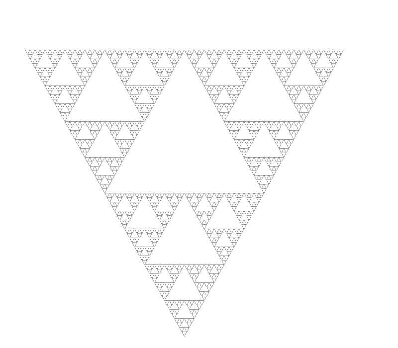
This one is called a Sierpinski Triangle or Sierpinski Gasket.
Consider this fractal definition:
{
    "axiom": "FX",
    "rules": {"X": "X+YF+",
              "Y": "-FX-Y"},
    "iterations": 15,
    "angle": 90.0,
    "forward": 3.0,
    "start_x": 280,
    "start_y": 200,
    "start_angle": 0,
    "width": 800,
    "height": 800
}
What exotic instructions will X and Y translate to? Nothing! Our turtle will ignore them completely. We don’t have to change a line of code and we’ll get the following fractal:
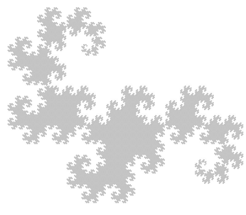
This is the famous Dragon Curve (it’s the one Michael Crichton used for “Jurassic Park”).
Explaining the Dragon Curve
The previous definition might need some explaining. I know I had no idea what was going on the first time I saw it. Let’s look at each iteration.
Iterating once gives us:
F+F+
Iterating twice gives us:
F+F++-F-F+
Iterating three times:
F+F++-F-F++-F+F+--F-F+
Four times:
F+F++-F-F++-F+F+--F-F++-F+F++-F-F+--F+F+--F-F+
Okay from here we should be able to see the pattern. Our basic pattern is always at right angles: we turn and repeat. The lines in black are from the previous iteration and the lines in blue are added in the current iteration. The effect of the rules is to repeat the entire pattern so far at a right angle to the previous pattern.
Here’s the first six iterations animated:
You can clearly see the ‘doubling’ effect of the rules.
The Hilbert Curve
The following definition will render a Hilbert Curve:
{
    "axiom": "L",
    "rules": {"L": "+RF-LFL-FR+",
              "R": "-LF+RFR+FL-"},
    "iterations": 7,
    "angle": 90.0,
    "forward": 5.0,
    "start_x": 100,
    "start_y": 700,
    "start_angle": 0,
    "width": 800,
    "height": 800
}
Which looks like this:
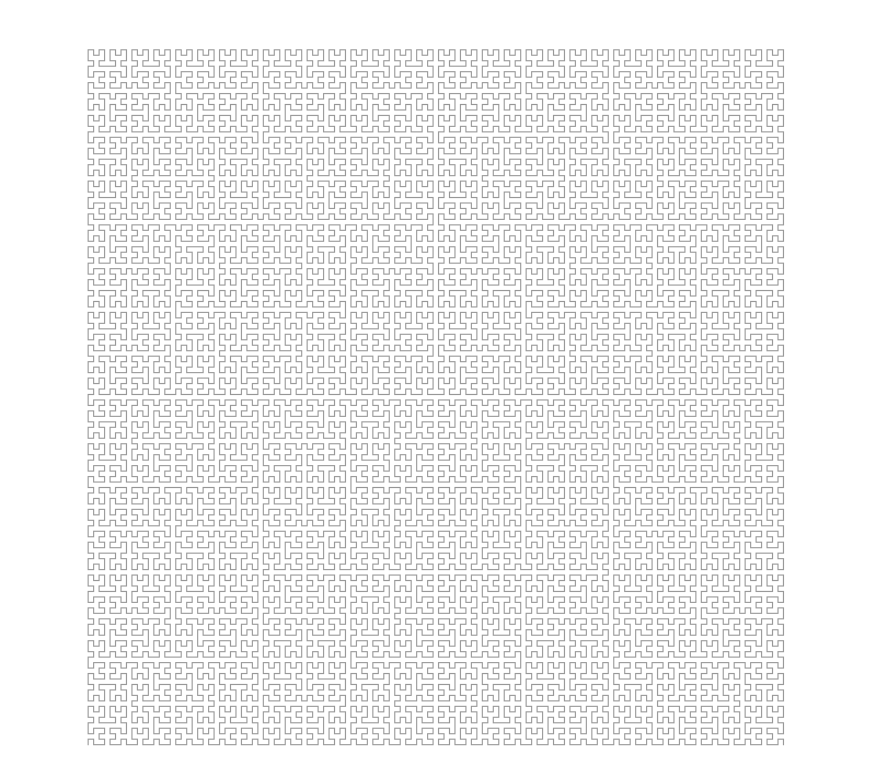
This is one of my favourite curves. It’s an example of something called a “Space Filling Curve”. If you keep iterating eventually you’ll cover the entire square area of the canvas. The interesting thing here is that this provides a way to map a 2D space into one dimension. We have a line, a 1 dimensional object, filling the 2 dimensional space. The following animation shows how this works:

There are lots of space filling curves (technically our Dragon curve is one too) but what’s interesting about the Hilbert curve is the following property: if two points are close together in 2D space then they will still be close together in 1D space. This is really useful and it’s worth reading the wikipedia page for more info.
I think that’s a fair place to end this post. Code is, as usual, on Gitlab. In the next post we’ll extend our L-systems to be able to generate plant-like fractals.