Fractals: the Mandelbrot Set

Sat 01 February 2020 by A Silent Llama

We’re going to temporarily set aside L-systems to look at a different type of fractal. As we’ve seen creating fractals involves repeating a process over and over again. We’ve seen this with simple drawings of triangles and squares and moved up to more complex patterns involving branching and randomness. We’re now going to take a detour in to the world of mathematical functions. I’m going to try and explain everything from the ground up - all I’m assuming is that you have some basic high school math.

Math Functions?

Repeating shapes makes intuitive sense but what can we achieve by repeating a math function? The example I’ve seen in several textbooks is one you’ve probably already played with. When you first get a calculator with a square root function a lot of people instinctively start pressing the button over and over again to see what happens. You’ll notice that eventually, no matter how big the starting number, you hit zero. This is an example of an iterated function. This should sound familiar - it’s exactly the same idea we’ve been using for our previously fractals - iterating the same process on itself.

Let’s start a new Rust project making sure we have the image library available:

$ cargo new mandelbrot

:::rust
// Cargo.toml
[dependencies]
image = "*"

Alright so which math functions are we going to try? I’m not going to jump straight into the fractal, I’m going to try and sneak up on it. We’ll start with the 1 dimensional case.

Escapism

For the heck of it let’s start with the function f(x) = x². Everyone who’s done high school math will be familiar with this one. We’re not going to draw the graph though - we’re going to focus on what happens when we iterate it.

Let’s pick a random starting number, say 4:

f(4) = 4² = 16

Now let’s iterate:

f(4) = 16; f(16) = 256; f(256) = 65536; f(65536) = 4294967296

Whoa, that’s going to get really big really fast. Let’s pick a different number, say, 0.4:

f(0.4) = 0.16; f(0.16) = 0.0256; f(0.0256) = 0.00065546; f(0.00065546) = a seriously small number

This one is the opposite - it just gets smaller and smaller.

One last one (literally):

f(1) = 1; f(1) = 1; f(1) = 1

This never goes anywhere.

We can see that there are three cases:

• The iterations get bigger and bigger. Some people like to say they blow up or escape.
• The iterations get smaller and smaller and eventually approach zero.
• The iterations stay constant.

We can simplify this down to two cases: either our iterations escape or they don’t. I’ve seen some texts describe the numbers that don’t escape as prisoner values which is a nicely evocative term.

One way of visualising the process is to imagine the multiplication stretching or squeezing our initial number. In general multiplying scales the number being multiplied.

You can imagine the numbers that escape are literally running away on the number line while the numbers that don’t are dragged back to the origin. You can practically hear the fingernails scraping on the number line floor.

Now we’re going to attempt to draw this so we can analyze the whole number line visually.

// main.rs
use image::{ImageBuffer, Rgb};
use std::path::Path;

fn main() {
    let width: u32 = 800;
    let height: u32 = 50;

    let mut imgbuf = ImageBuffer::from_pixel(width, height, Rgb([255, 255, 255]));

    for x in 0..width {
        // Need to iterate here:
        // -- Todo --
        imgbuf.put_pixel(x, 25, image::Rgb([0, 0, 0]));
    }

    imgbuf
        .save(&Path::new("rendered.png"))
        .expect("Unable to save image");
}

Okay - we’ve set up an image and we’re going to walk across the width of the image. Iterating our function only produces a single value so we fix our y coordinate to 25 for now. We’re going to analyze the iterations in the following way:

• If after iterating a point x escapes then we colour that point in white.
• For the points that don’t escape (the prisoner points) we colour the point in black.

We’re hoping that whatever visual turns up it’ll help us understand our function a little more. So, how do we tell whether a point escapes or not? We’re going to use a rule of thumb (we’re computer people not mathematicians!). We can see from the examples above that points bigger than 1 escape so we’ll just say that if, after iterating, the output is bigger than 1 then we know the value will escape and if it’s smaller or equal to 1 then it won’t. We’ll call this number our escape threshold.

Here we go:

// main.rs
use image::{ImageBuffer, Rgb};
use std::path::Path;

fn main() {
    let width: u32 = 800;
    let height: u32 = 50;

    let mut imgbuf = ImageBuffer::from_pixel(width, height, Rgb([255, 255, 255]));
    let max_iterations = 10;
    let escape_threshold = 1.0;

    for x in 0..width {
        let mut iteration = 0;
        let mut iterated_value = x;

        // We check for both the escape_threshold and max_iterations so we can
        // bail out early the moment we exceed the threshold. This isn't important
        // in this 1 dimensional case but it helps when we move to 2D.
        while iterated_value <= escape_threshold && iteration < max_iterations {
           iterated_value = iterated_value * iterated_value;
           iteration += 1;
        }

        // We can only hit our max_iterations value if we *don't* escape:
        if iteration == max_iterations {
           // The entire image is white by default so we
           // only need to worry about colouring in the
           // case where we don't escape:
           imgbuf.put_pixel(x, 25, image::Rgb([0, 0, 0]));
        }
    }

    imgbuf
        .save(&Path::new("rendered.png"))
        .expect("Unable to save image");
}

If you try and run this we’ll get an error! What’s the problem? Well - we’re scanning over the width of our image but that means our x is only ever going to hit the sequence 1, 2, 3 up until our width. We’re missing all the real numbers in between and we’re going far enough that we’re multiplying numbers big enough to overflow our iterated_value.

What we need to do is find some way to map our width onto the number line that we’re analysing. For now let’s say we only really want to analyse what happens to our function for the numbers from -2.0 to 2.0. We’ll call these our start and end values:

// main.rs
// -- snip --
let max_iterations = 10;
let start: f64 = -2.0;
let end: f64 = 2.0;
// -- snip --

From this we can work out that the width on the number line by calculating the absolute value of the difference between end and start:

let number_line_width = (end - start).abs();

If we divide our number_line_width with the width of our image we’ll essentially find out how big a step we need to take on the number line for each step in the image. Think of the image like a window into the number world - we’re just working out what portion of the number line we’re looking at. If we liked we can zoom in by making our start and end closer together or zoom out by making our start and end further apart.

// This fits the number_line_width into our image width:
let step: f64 = number_line_width / width as f64;

We’re working with small numbers here so we need to tell Rust to use floating point numbers. Now when we iterate we use our start value as the first value to iterate. We know that each pixel on the image represents a size step on the number line so we need to multiply our step by our current x value to find out how far we are on the number line.

// main.rs
for x in 0..width {
    let mut iteration = 0;
    // Convert our x on the image to a point on the number line:
    let mut iterated_value = start + (x as f64 * step);

    while iteration < max_iterations {
       iterated_value = iterated_value * iterated_value;
       iteration += 1;
    }

    if iterated_value < escape_threshold {
       imgbuf.put_pixel(x, 25, image::Rgb([0, 0, 0]));
    }
}

This produces the following exciting image:

Alright, maybe not so exciting. We’ve managed to draw a line without needing the Bresenham algorithm though. Good for us! We can see something interesting though - there’s only a small section of this function that doesn’t escape. This makes sense - any number bigger than 1 will keep getting bigger so the only section that can’t escape are the numbers between -1 and 1.

Escaping in 2D

Lines are boring. What happens if we move into 2D space? We want to do the same thing f(x) = x² but how? If we try the equation: f(x,y) = x² + y² we notice that it’s output is a single number but its input is two numbers. How are we supposed to iterate it?

What we’re going to need is something 2 dimensional that when multiplied with itself produces another 2 dimensional thing. Then we can write our equation as f(something) = something². We just need to define this elusive something. What we’re really looking for is a 2 dimensional number.

2 Dimensional Numbers

Let’s look back to our very first equation: f(x) = x². Mathematicians have spent years looking at equations like that trying to work out their solutions. For example if f(x) = 4 then we know:

f(x) = 4

∴ x² = 4

∴ x = √4

∴ x = 2 or x = -2

What about the following?

f(x) = -1

∴ x² = -1

∴ x = √-1

Whoops! We can’t get a square root of a negative number. A negative times a negative is always positive, there’s no way we can find a number multiplied by itself and still get a negative.

This is annoying for mathematicians and for good reason. You might notice that when we can solve this equation that there are 2 valid solutions. It’s irksome that a particular set of numbers provides no solution at all. Mathematicians fixed this problem by introducing a new number: i.

We define i as follows: i * i = -1 and therefore i = √-1. You might think this is crazy - how can we just go ahead and declare the existence of an entirely new number, especially one that seems to defy the previous laws of math? Well - we’ve done it before. Think of the sum 3 - 4. That’s technically impossible too. There’s no way we can subtract more than we have. But mathematicians solved that by introducing a new type of number: -1. We know what it means: it means I owe you one.

In order for this to work mathematicians declared that from now on we have a new mixed type of number. It mixes our ordinary numbers with these new imaginary numbers (which is what i stands for). They call these numbers complex numbers, not because they’re difficult but because they’re no longer simple. A simple thing has only one part - these numbers have two parts: a Real part and an Imaginary part. Now we can get an entire Imaginary number line by simply adding up i. We can start with i and then have 2i, 3i, -i etc…

If the Real number line is the one we’ve always used where is the Imaginary one? Well - it’s directly opposed to the Real line and hence it’s perpendicular to it:

We now have our 2 dimensional number. It’s important to note that the numbers don’t mix - if we add 1 to i we get the number 1 + i. Similarly if we subtract i we get 1 - i. The imaginary part lives in a seperate world from the real part but the combination allows us to find a single complex number for any point in the 2D plane. We can find the point like this: walk our x real units on the real number line and then walk i units on the imaginary number line.

In the above diagram we can see the imaginary components in green and the real components in blue.

How does multiplication work for Complex Numbers?

So we already saw for our everyday numbers that we can use this idea of stretching or squeezing to define multiplication. But what does multiplication for imaginary numbers do?

Let’s multiply 1 by i. If we have one of i then we have i so 1 * i = i. Multiplying again gives i * i which is -1 (by definition). Multiplying again gives: -1 * i which is -i. One last multiplication brings us back to 1.

Visually this looks like:

If we multiply by i we rotate 90°. In general the imaginary components of a complex number rotate by some angle when we multiply. We can write our complex numbers in a different way - if we think of a complex number as being connected to the origin by a line we can create a triangle with some hyptoneuse and angle. Multiplying will then stretch one number by the hyptoneuse of the other and will then add the angles:

Back to our code. Lucky we don’t need to implement complex numbers (this post is long enough already) - Rust has a library ready for us:

// Cargo.toml
[dependencies]
num_complex = "0.2"

Now we can use them in our program:

// main.rs
// -- snip --
use num_complex::Complex64;

let width: u32 = 800;
let height: u32 = 800;
let aspect_ratio: f64 = width as f64 / height as f64;

// The further in we zoom the more iterations are required - we make this
// an unsigned 64 bit number to handle just about anything you feel like
// throwing at it.
let max_iterations: u64 = 30;
let escape_threshold = 1.0;

// Our starting point - this is the top left corner of
// the 'window' into the fractal world.
let start_x: f64 = -2.0;
let start_y: f64 = -2.0;

// delta_x is the width of our window.
let delta_x = 4.0;
let delta_y = delta_x / aspect_ratio;

let step_x: f64 = delta_x / width as f64;
let step_y: f64 = delta_y / height as f64;

for x in 0..width {
    for y in 0..height {
        let mut iteration = 0;

        let mut c = Complex64 {
           re: start + (x as f64 * step_x),
           im: start + (y as f64 * step_y)
        };

        while c.norm_sqr().sqrt() < escape_threshold && iteration < max_iterations {
           c = c*c;
           iteration += 1;
        }

        if iteration == max_iterations {
           imgbuf.put_pixel(x, y, image::Rgb([0, 0, 0]));
        }
    }
}

The difference is we’re now going to scan over our entire image instead of just a line so we need to add a second for loop over the image height. Just about everyone renders these images as squares but I’ve added in the calculations for making rectangular images (separating out the x step from the y step and making sure we maintain the same aspect ratio so the image doesn’t become distorted).

One extra twist is for the escape threshold. Previously we could just check if the value we iterated was smaller than the threshold but we have a problem now: Complex numbers don’t have an order! It’s easy to order things on a line but how would you order points in space?

The solution is to re-examine what we were actually doing: when checked our escape threshold in the first program what we were actually doing was comparing the distance of that point from the origin. Since squaring the number always makes it positive we didn’t need to worry about the negative case. So - can we do the same, can we compare the distance of a complex number from the origin?

Pythagoras to the rescue! Of course we can - the distance of a complex point from the origin is simply the length of the hyptoneuse of the triangle you make by connecting the real point on the Real axis, the imaginary point on the y axis the origin to the point itself. E.g.:

The complex number library we are using has a function to work this out for us: norm_sqr(). We just need to then take the square root and we have our distance from the origin. We can use an escape threshold of 1.0 again - just as with the 1 dimensional case we saw that every number greater than 1 escapes.

We now get:

This should make sense and come as something of a relief - from high school we know that the equation for a circle is x² + y² = r² and, intuitively, squaring our complex numbers feels like we should get something circular out of it. Complex multiplication stretches and squeezes in the same way as our normal Real multiplication did in our first 1 dimensional example. So - anything within the boundary of the circle should get squeezed down to our zero point and everything else should escape.

Now, I know what you’re thinking. This is a really long blog post and we haven’t even drawn a fractal yet. Well - we’re going to add one last wrinkle to our ‘escape analysis’. Instead of just iterating the square of each point we’re going to give each point a little bump. Let’s say our starting point is some complex number c. We’ll then iterate on the equation z² + c where z is a complex number that starts from 0. This is almost the same as the equation that generated our circle so its worth trying to guess what will happen. After 1 iteration we’ll have c² just like the first case. But now - we add c back on every iteration. This has the effect of moving our point every iteration. When I first saw it I wondered if it might make our circle smaller. If we keep adding in c it might make it easier for numbers to escape. I then wondered if it might add some bumps to the circle since c might move back into the no escape zone. Think about what you expect the result to be. We can also see that we need to use a larger escape threshold since iterating 2i gives us the sequence -2, 2, -2 etc - the escape threshold must be bigger than 2.

Before we render the whole image here’s a quick diagram illustrating things. This shows the paths particular points travel as we iterate them. You can see how the red and black points escape. The pink point is constant - travelling the same path over and over again. The green point spirals into itself.

We’re ready to do the escape analysis. Let’s draw it:

// main.rs
// -- snip --
let escape_threshold = 2.0;
// -- snip --
for x in 0..width {
    for y in 0..height {
        // c is the point in the complex plane that matches our current
        // position in the image:
        let c = Complex64 {
            re: start + (x as f64 * step_x),
            im: start + (y as f64 * step_y)
        };

        let z = Complex64 { re: 0.0, im: 0 };

        while z.norm_sqr().sqrt() < escape_threshold && iteration < max_iterations {
           z = z*z + c;
           iteration += 1;
        }

        // -- snip --
    }
}

And here’s the what we get:

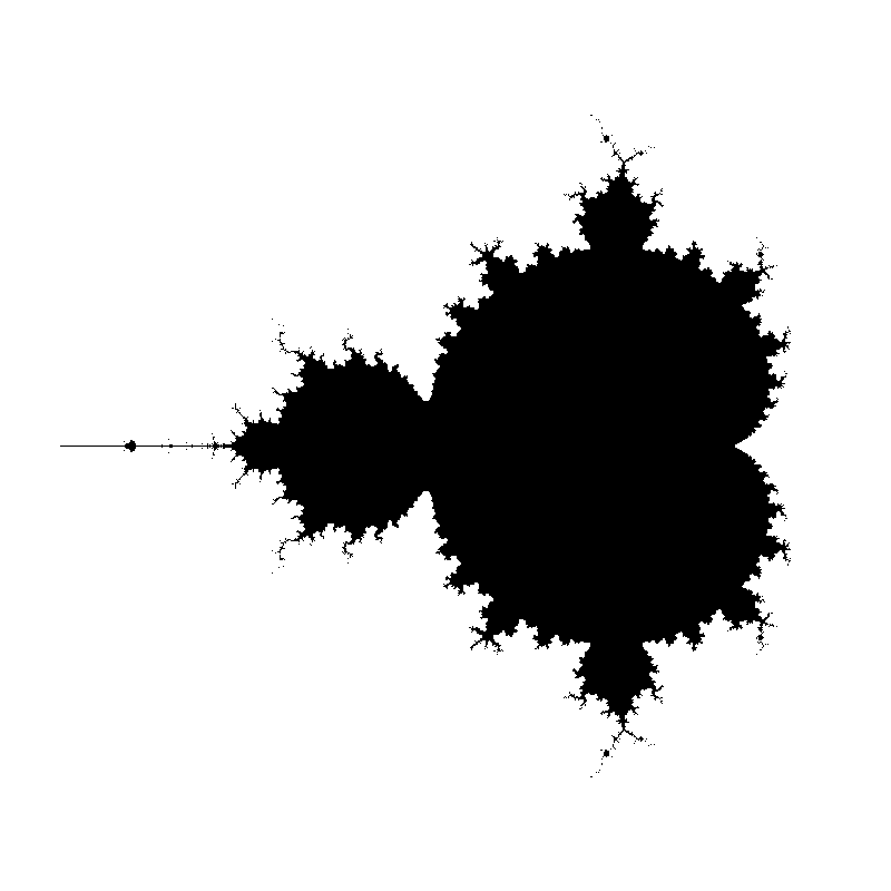
Well - there are definitely a few bumps! This is one of the most famous fractals of all: the Mandelbrot Set. All the numbers that don’t escape, the prisoner numbers, are in the set and coloured black. The incredible thing is that this picture can be zoomed in indefinitely. Everywhere you look you’ll see a complex mathematical structure.

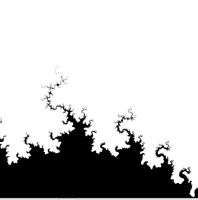
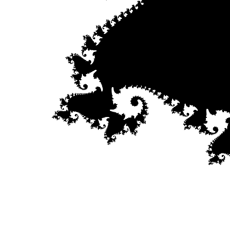
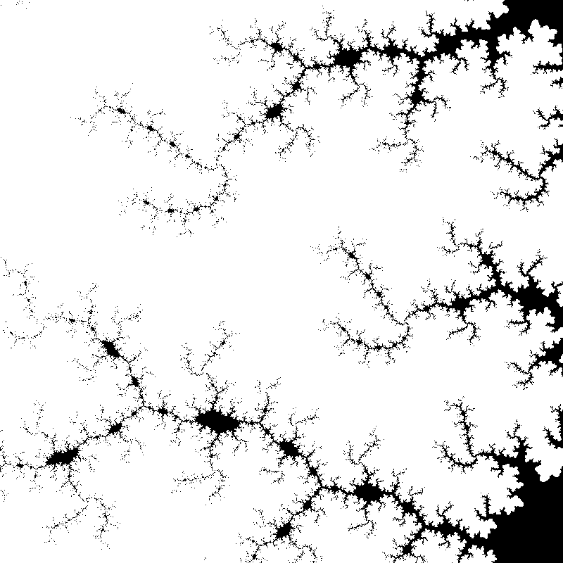
In fact let’s zoom in so we can see some of the structure - it’s amazing what we can find inside this fractal (remember you can zoom by setting the start_x and start_y and delta_x values. Remember though - the more you zoom the more iterations you’ll need to check if a point escapes or not):

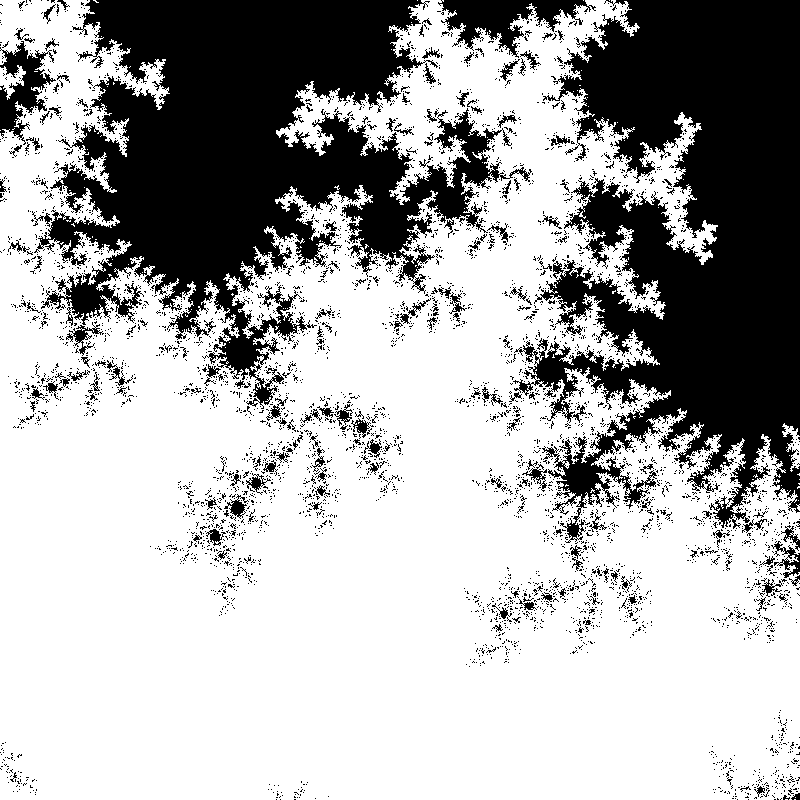
It’s incredible that all this is because of a simple equation: z = z² + c but it is. You might ask, though, why don’t these images look as colourful as the ones you usually see on the internet? Well - in the next post I’ll show you another type of fractal (the Julia Set) and we’ll work on colouring them so we won’t be too embarrased to show them our friends.

The code is on Gitlab as usual.

References

Wikipedia